Indexing

Data Science 310

Boston University

Efficient Data Access

How can we find items quickly in a table?
Recall that the time consuming operations in a database are disk accesses
- We will consider a disk access to be reading a single block, or reading a sequence of blocks as a page
- This is because the time needed to read from disk is dominated by the “seek” time – moving the head
The simplest case to consider is looking up a record by a key

select name from employee where employee_id = '142552'

To do this efficiently we will use an index

Index Structures

An index structure stores (key, value) pairs.
- also known as a dictionary or map
- we will sometimes refer to the (key, value) pairs as items

The index allows us to more efficiently access a given record.
- quickly find it based on a particular field
- instead of scanning through the entire collection to find it

A given collection of records may have multiple index structures:
- one clustered or primary index
- some number of unclustered or secondary indices

Clustered/Primary Index

The clustered index is the one that stores the full records.
- also known as a primary index, because it is typically based on the primary key

If the records are stored outside of an index structure, the resulting file is sometimes called a heap file.
- managed somewhat like the heap memory region

Unclustered/Secondary Indices

In addition to the clustered/primary index, there can be one or more unclustered indices based on other fields.
- also known as secondary indices

Example: Customer(id, name, street, city, state, zip)

primary index:
(key, value) = (id, all of the remaining fields in the record)

a secondary index to enable quick searches by name
(key, value) = (name, id) does not include the other fields!

We need two lookups when we start with the secondary index.
- example: looking for Ted Codd’s zip code

search for 'Ted Codd' in the secondary index
→ '123456' (his id)

search for '123456' in the primary index
→ his full record, including his zip code

B-Trees

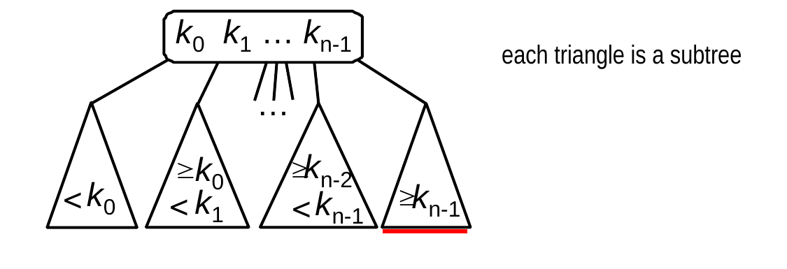
A B-tree of order m is a tree in which each node has:
- at most 2m items (and, for internal nodes, 2m + 1 children)
- at least m items (and, for internal nodes, m + 1 children)

exception: the root node may have as few as 1 item

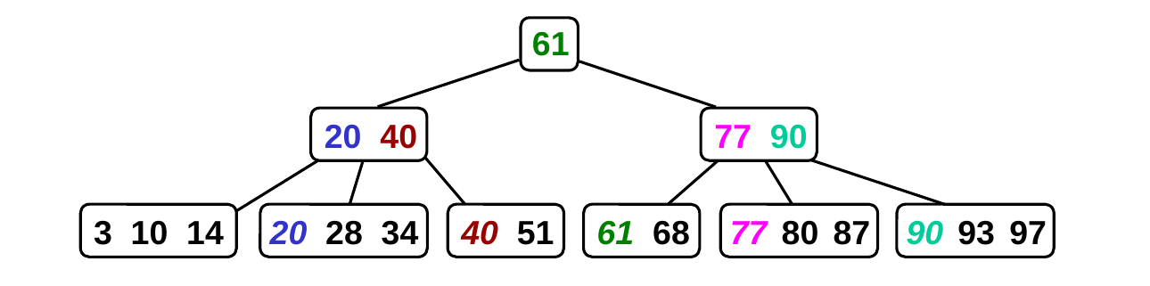
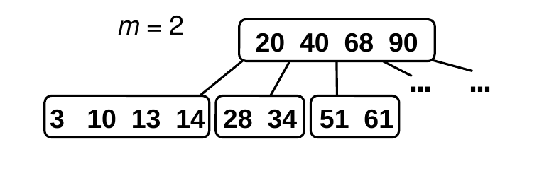
Example: a B-tree of order 2 (we’re just showing the keys)

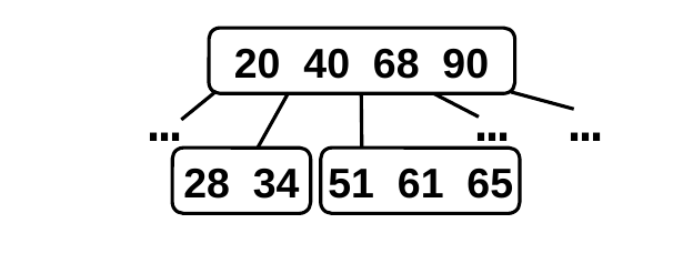
A B-tree has perfect balance: all paths from the root node to a leaf node have the same length.

Search in B-Trees

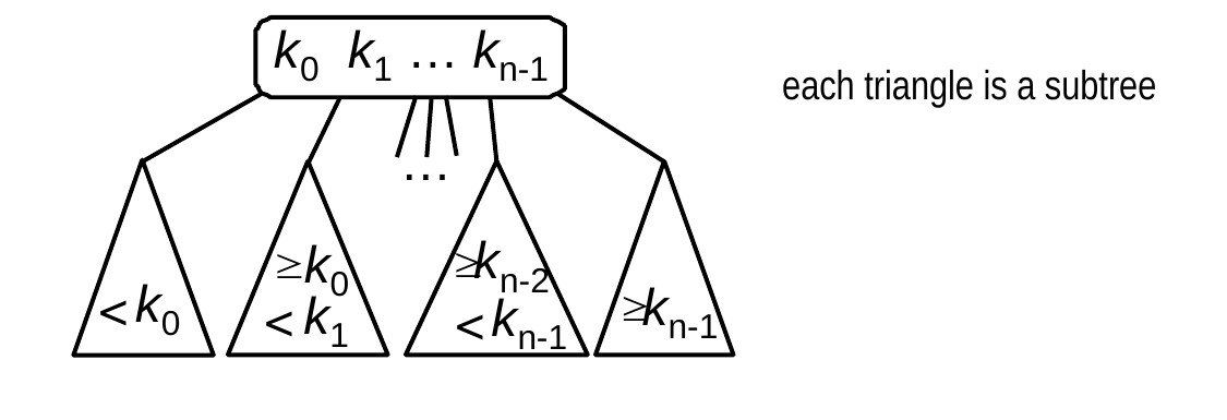
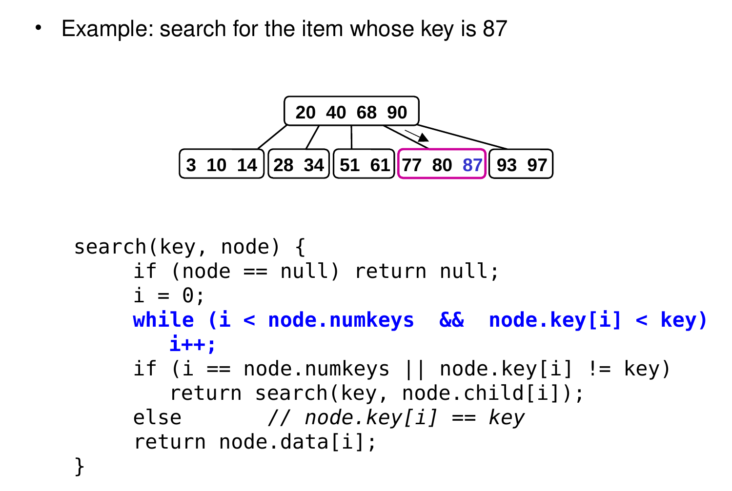
A B-tree is a search tree.
- like a binary search tree, but can have more keys per node

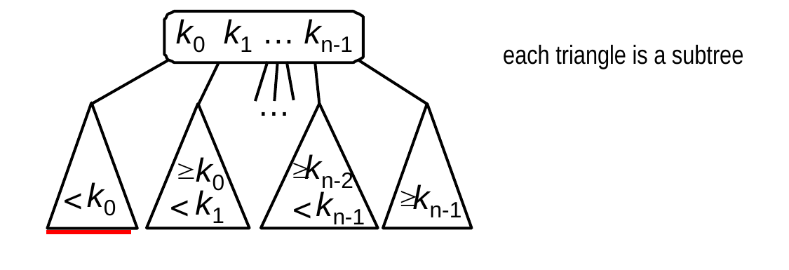
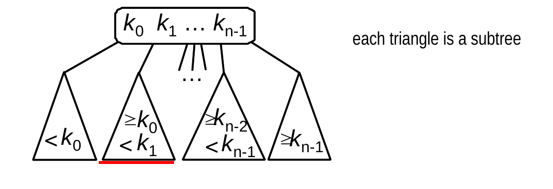
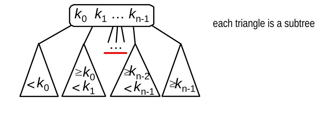
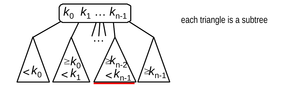
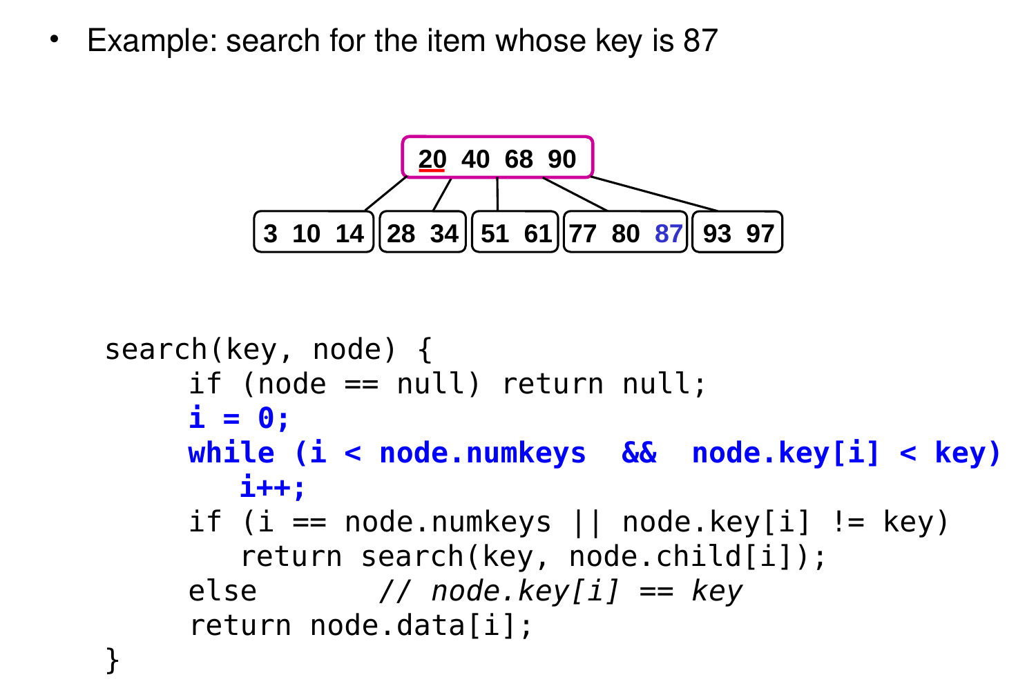
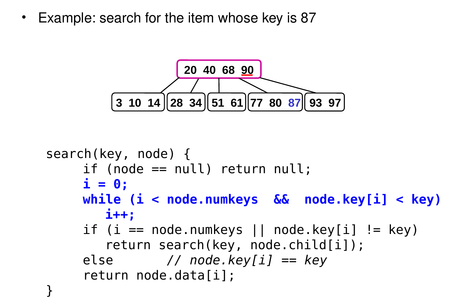
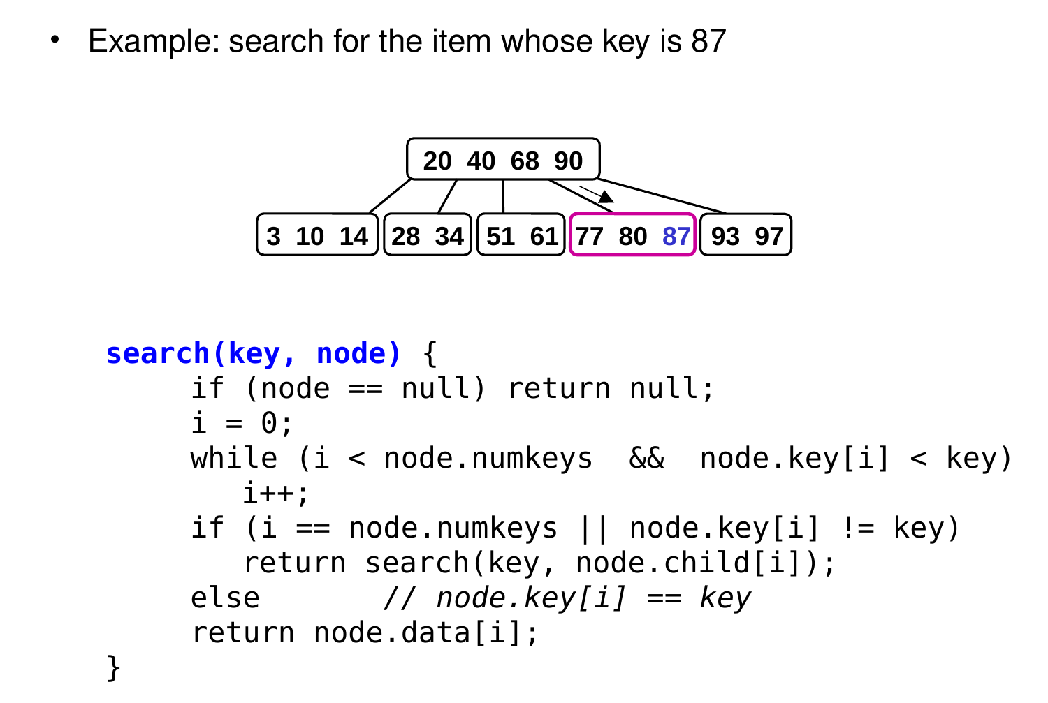
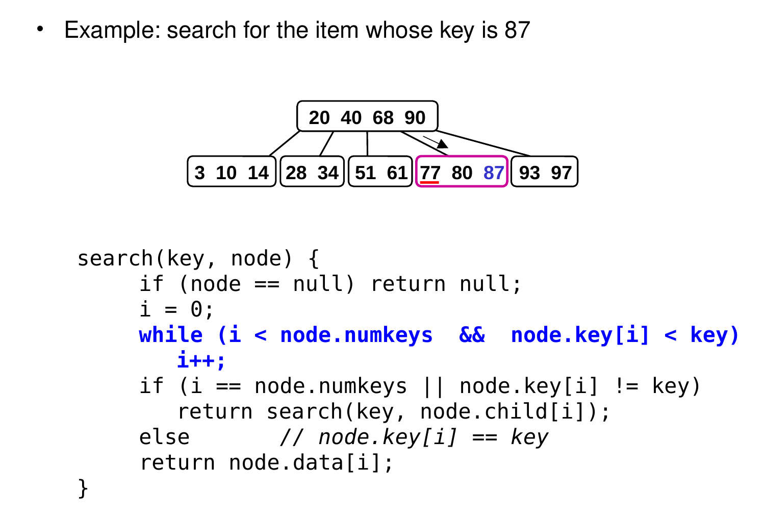
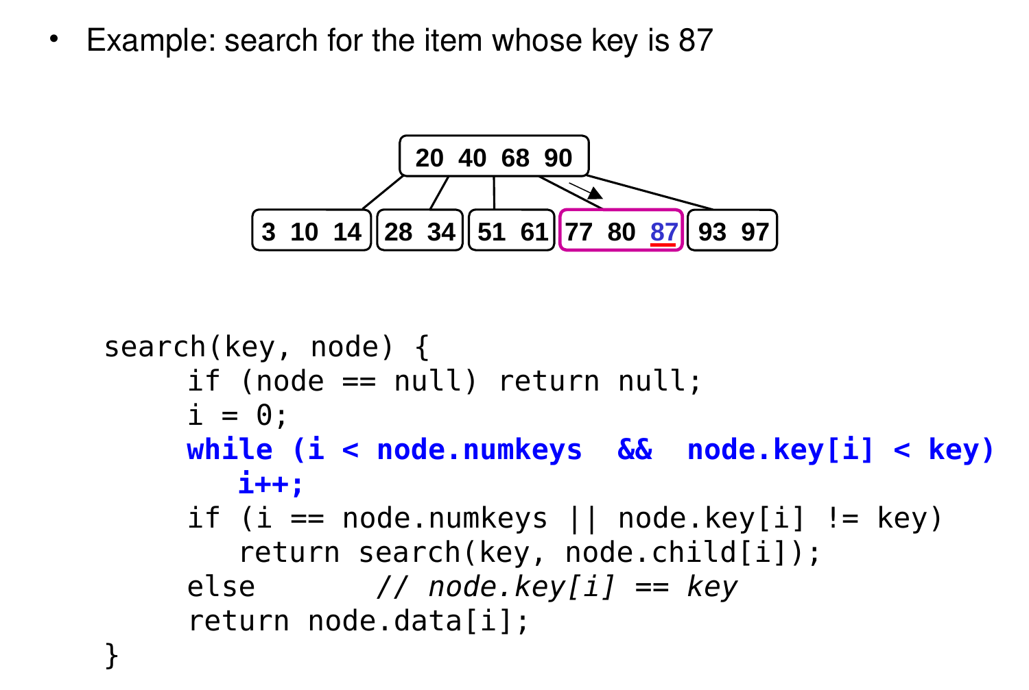
When searching for an item whose key is k, we never need to enter more than one of the subtrees of a node.

Search in B-Trees (cont.)

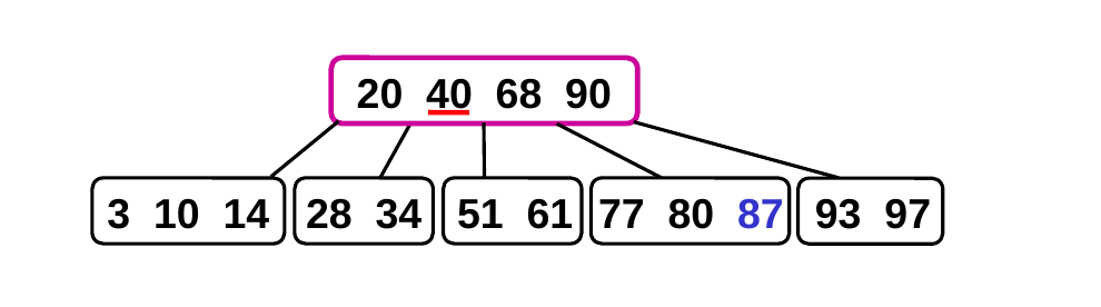
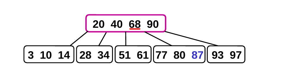
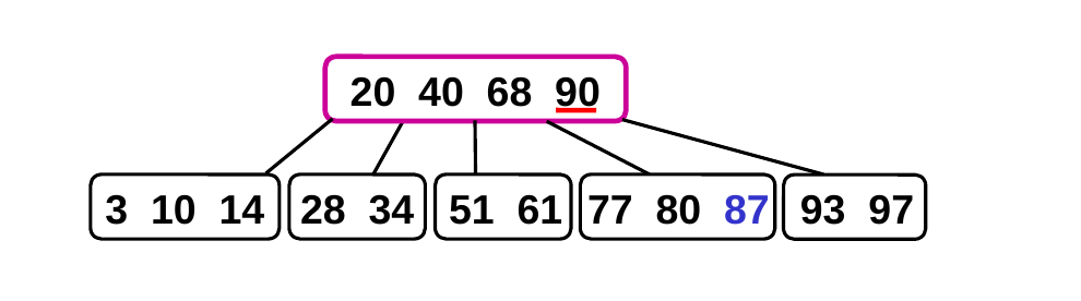
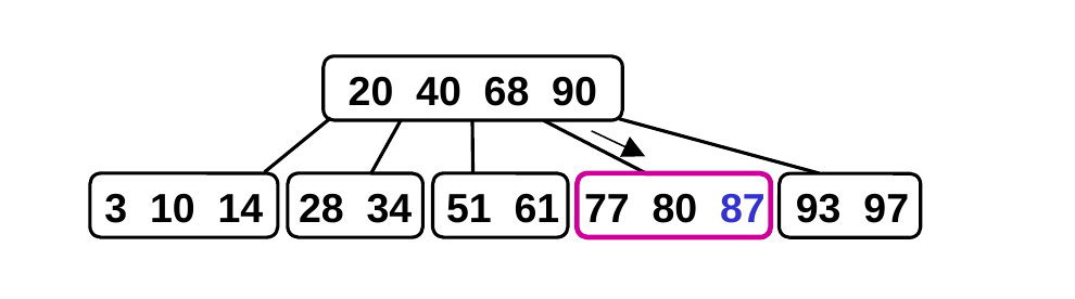
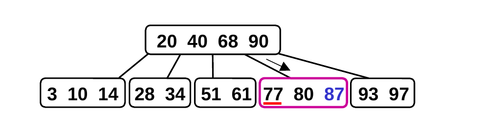
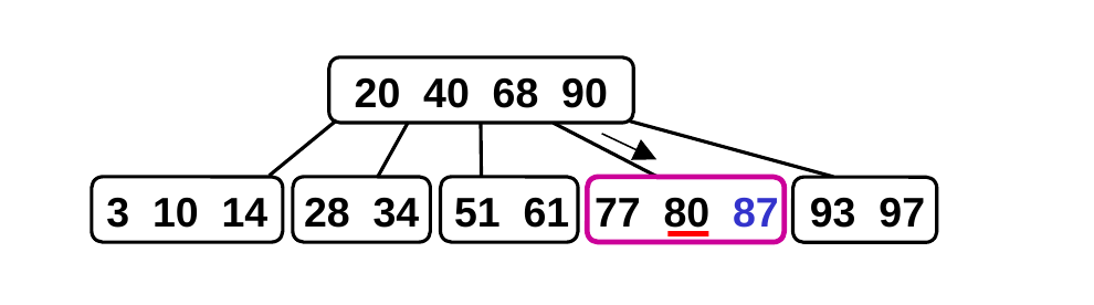
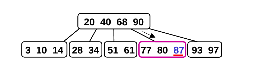
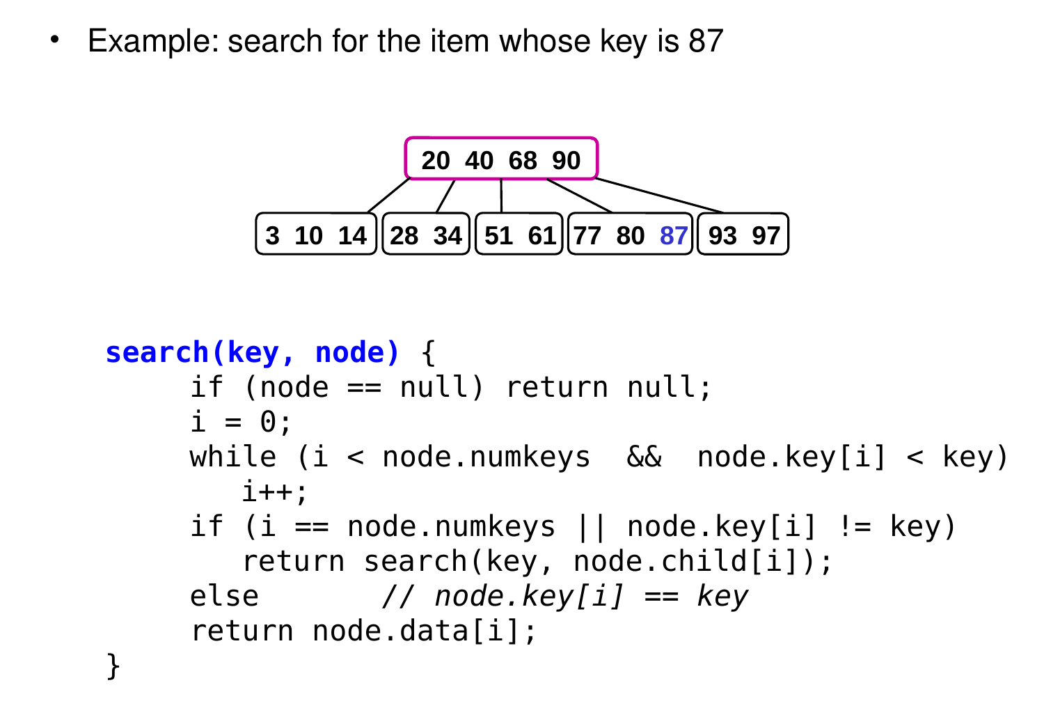
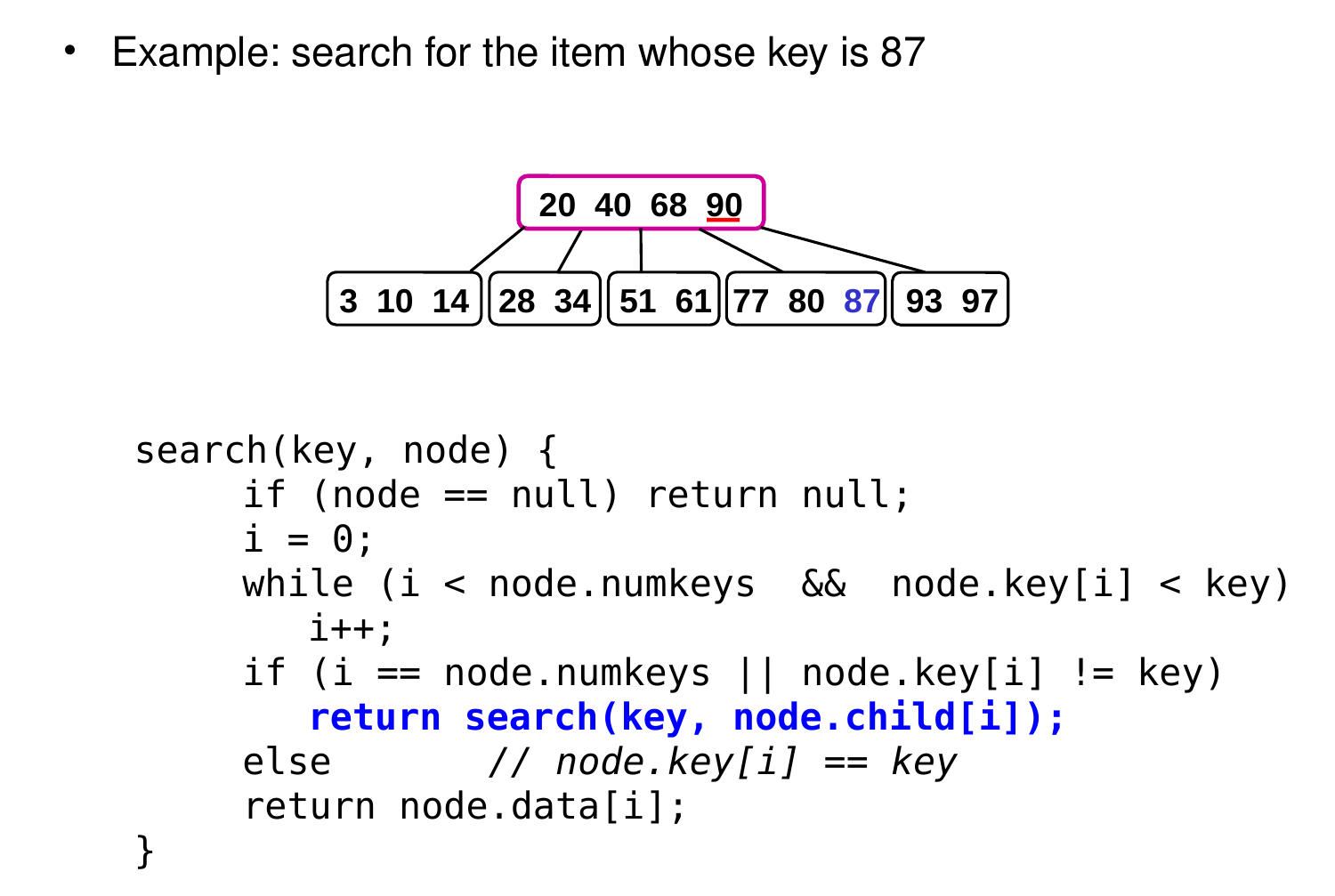
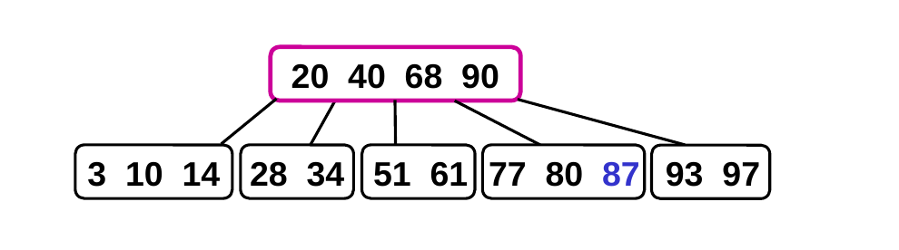
Example: search for the item whose key is 87

Search in B-Trees (cont.)

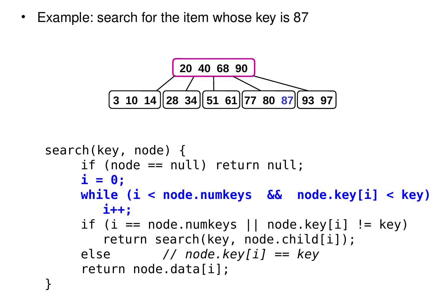
Example: search for the item whose key is 87

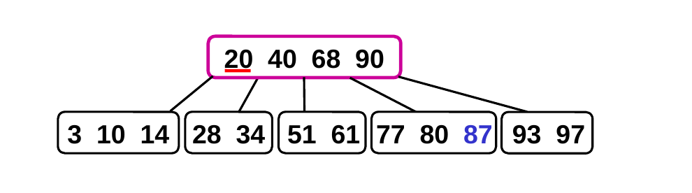
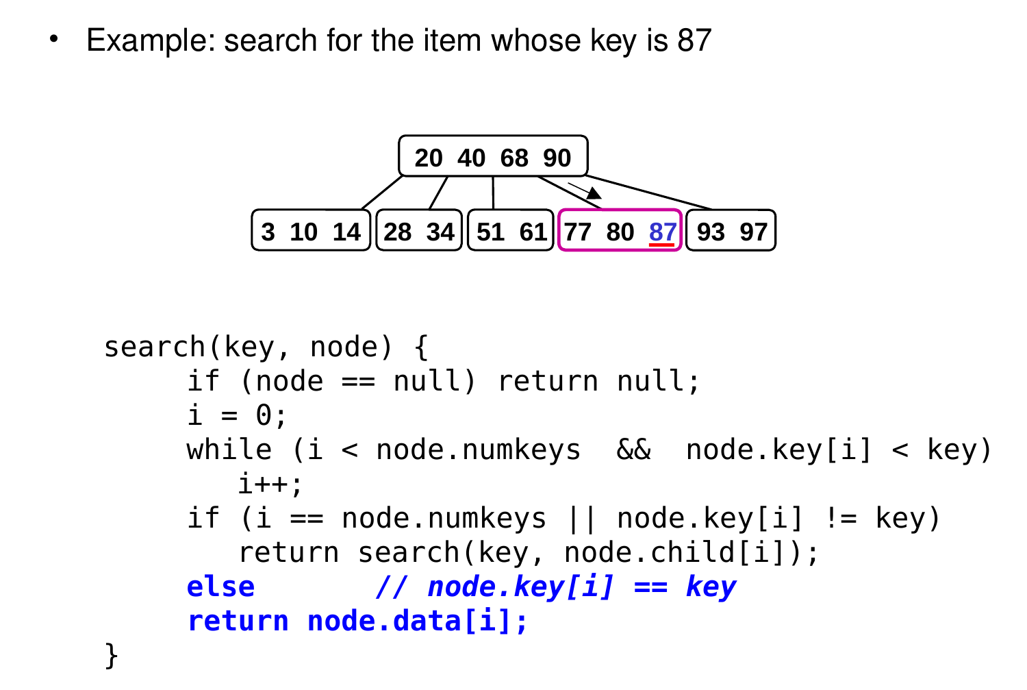
Here’s pseudocode for the algorithm:

search(key, node) {
    if (node == null) return null;
    i = 0;
    while (i < node.numkeys  &&  node.key[i] < key)
        i++;
    if (i == node.numkeys || node.key[i] != key)
        return search(key, node.child[i]);
    else       // node.key[i] == key
        return node.data[i];
}

Insertion in B-Trees

Algorithm for inserting an item with a key k:
- search for k until you reach a leaf node
- if the leaf node has fewer than 2m items, add the new item to the leaf node
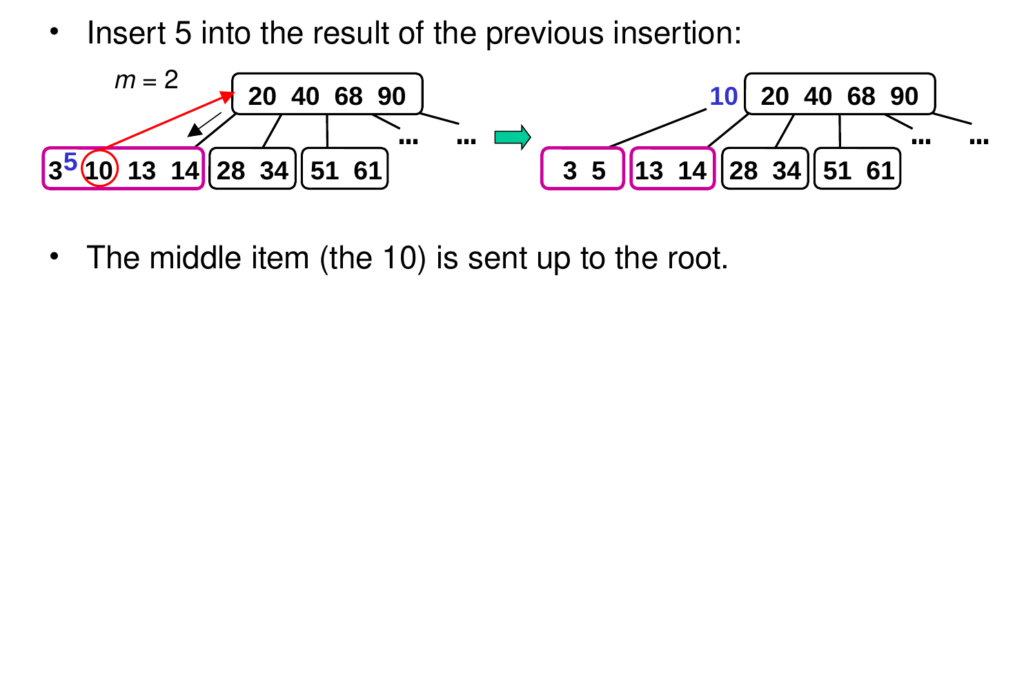
- else split the node, dividing up the 2m + 1 items:
  - the first/smallest m items remain in the original node
  - the last/largest m items go in a new node
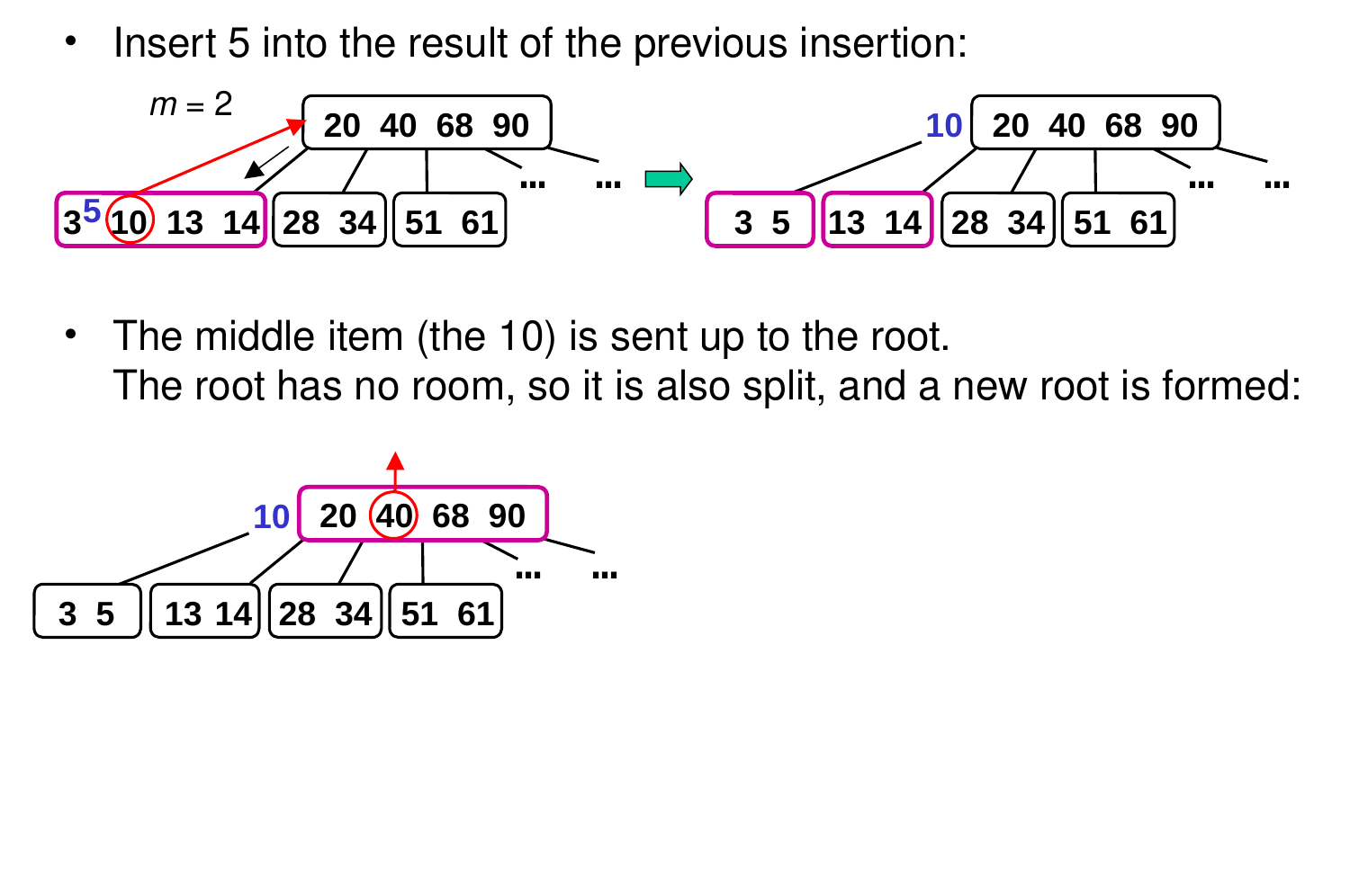
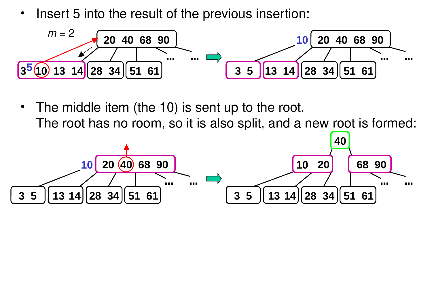
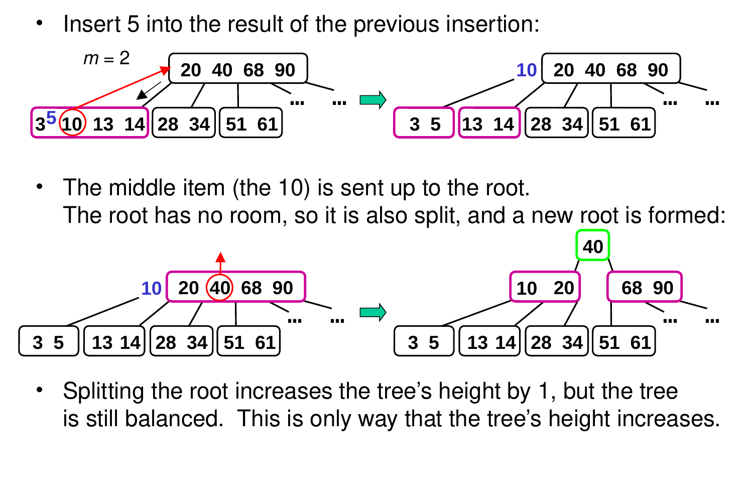
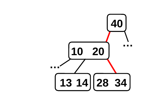
  - send the middle item up and insert it (and a pointer to the new node) in the parent

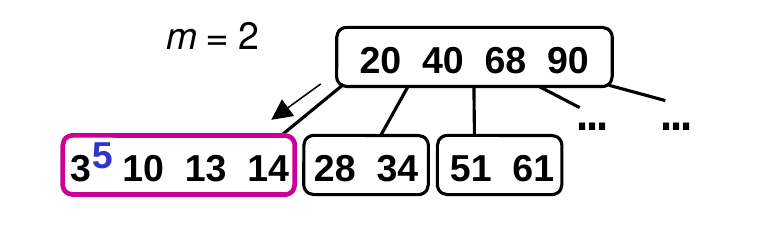
Example of an insertion without a split: insert 13

Example

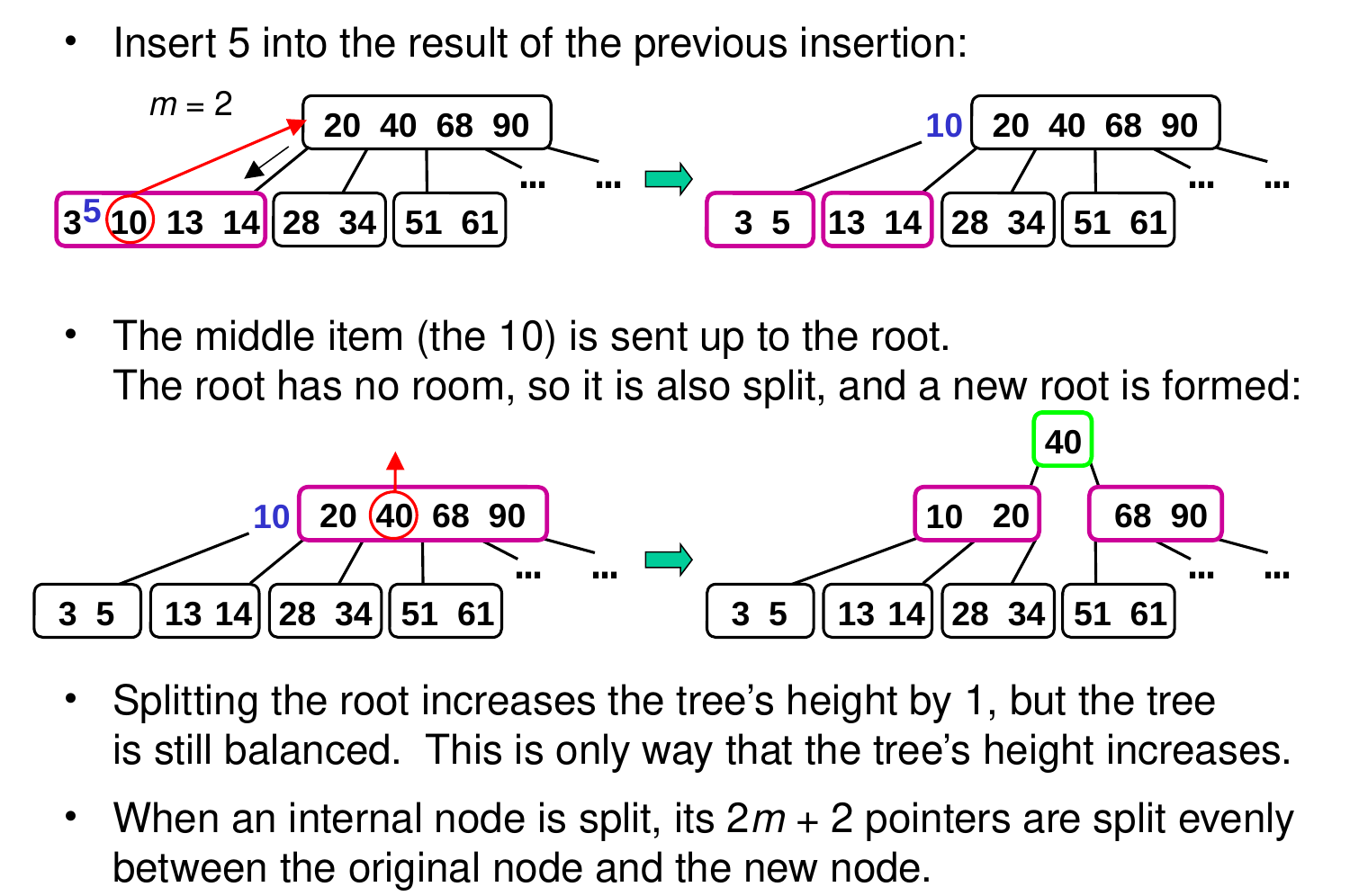
Insert 5 into the result of the previous insertion:

What happens?

Insert 5 into the result of the previous insertion:

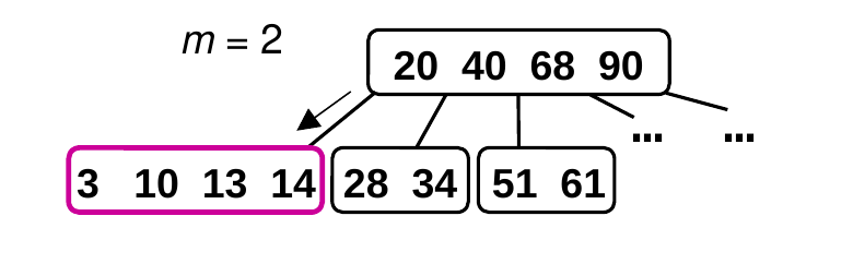
A. 5 stays in that leaf, and no splits occur

B. 5 stays in that leaf, and 10 is sent up as part of a split ← correct

C. 5 stays in that leaf, and 14 is sent up as part of a split

D. 5 is sent up as part of a split

Splits in B-Trees

Other Details of B-Trees

Each node in the tree corresponds to one page in the corresponding index file.
- child pointers = page numbers

Efficiency: In the worst case, searching for an item involves traversing a single path from the root to a leaf node.

# of nodes accessed <= tree height + 1

each internal node has at least m children
→ tree height <= log_mn, where n = # of items

→ search and insertion are O(log_mn)

To minimize disk I/O, make m as large as possible.

but not too large!
if m is too large, can end up with items that don’t fit on the page and are thus stored in separate overflow pages

B+Trees

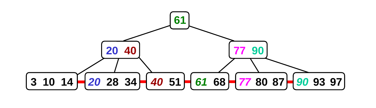
A B+tree is a B-tree variant in which:
- data items are only found in the leaf nodes
- internal nodes contain only keys and child pointers
- an item’s key may appear in a leaf node and an internal node
Example: a B+tree of order 2

B+Trees (cont.)

Advantages:
- there’s more room in the internal nodes for child pointers
  - why is this beneficial?

→ shorter tree → less disk I/O

because all items are in leaf nodes, we can link the leaves together to improve the efficiency of operations that involve scanning the items in key order (e.g., range searches)

Differences in the Algorithms for B+Trees

When searching, we keep going until we reach a leaf node, even if we see the key in an internal node.

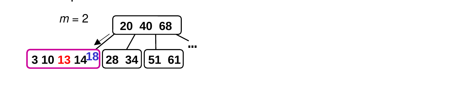
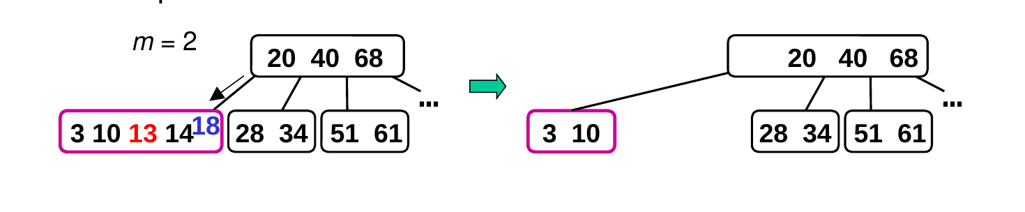
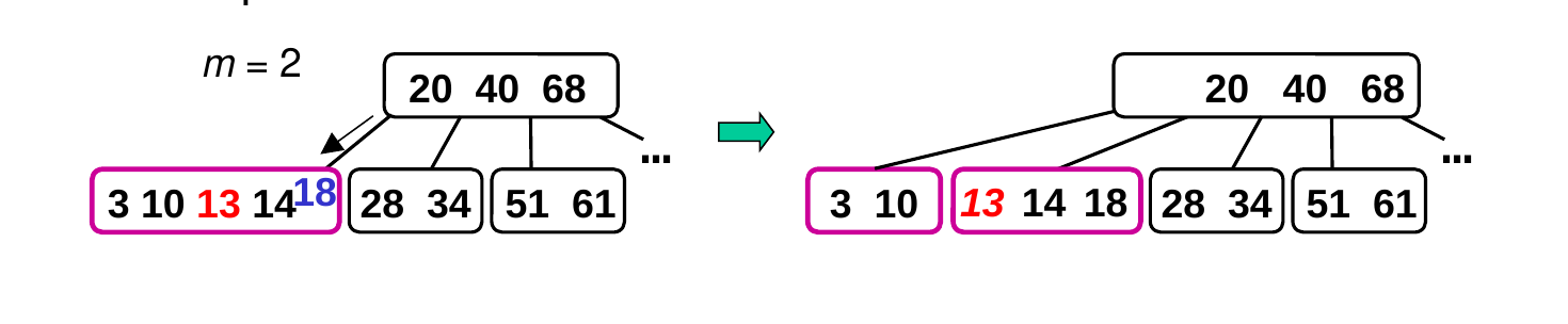
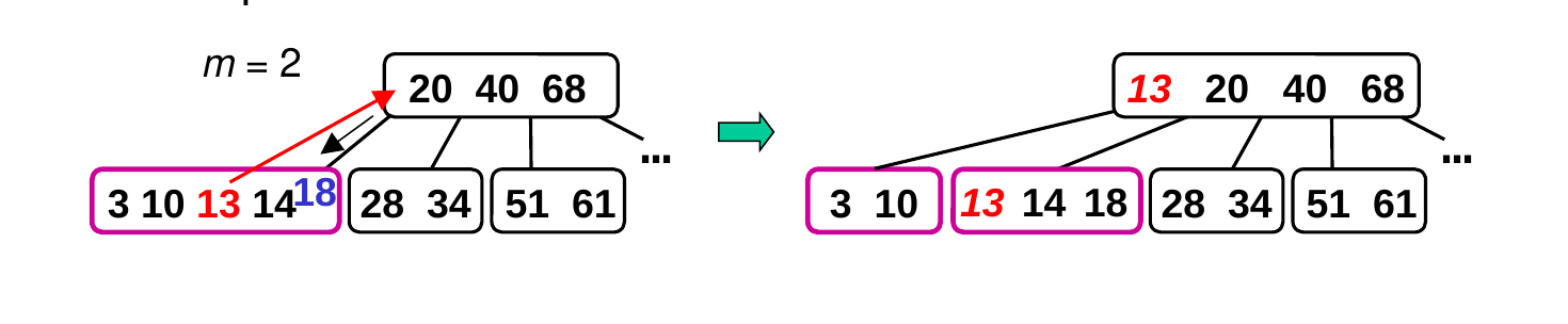
When splitting a leaf node with 2m + 1 items:

the first m items remain in the original node as before

all of the remaining m + 1 items are put in the new node, including the middle item

the key of the middle item is copied into the parent

why can’t we move up the entire item as before?
in a B+tree, all items are in leaf nodes!

Example: insert 18

Differences in the Algorithms for B+Trees (cont.)

Splitting an internal node is the same as before, but with keys only:
- first m keys stay in original node, last m keys go to new node
- middle key is sent up to parent (not copied)

Deletion in B-Trees and B+Trees

Search for the item and remove it.
If a node N ends up with fewer than m items, do one of the following:

if a sibling node has more than m items, take items from it and add them to N

if the sibling node only has m items, merge N with the sibling

If the key of the removed item is in an internal node, don’t remove it from the internal node.
- we need the key to navigate to the node’s children
- can remove when the associated child node is merged with a sibling

Some systems don’t worry about nodes with too few items.
- assume items will be added again eventually

Ideal Case: Searching = Indexing

The ideal index structure would be one in which:
- key of data item = the page number where the item is stored
In most real-world problems, we can’t do this.
- the key values may not be integers
- we can’t afford to give each key value its own page

To get something close to the ideal, we perform hashing:
- use a hash function to convert the keys to page numbers
  h('hello') → 5

The resulting index structure is known as a hash table.

Hash Tables: In-Memory vs. On-Disk

In-memory:
- the hash value is used as an index into an array

depending on the approach you’re taking, a given array element may only hold one item

need to deal with collisions = two values hashed to same index

On-disk:
- the hash value tells you which page the item should be on

because pages are large, each page serves as a bucket that stores multiple items

need to deal with full buckets

Static vs. Dynamic Hashing

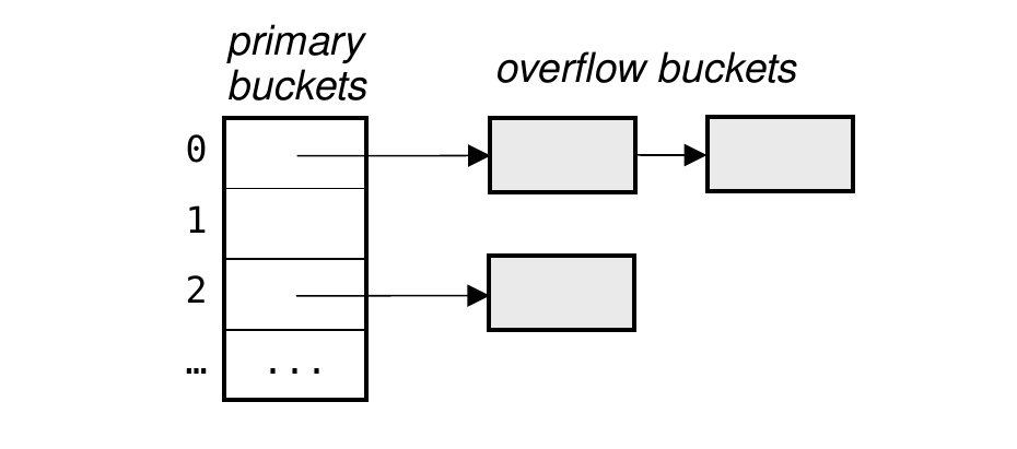
In static hashing, the number of buckets never changes.
- if a bucket becomes full, we use overflow buckets/pages

why is this problematic?
accessing an overflow bucket may require an extra disk read

In dynamic hashing, the number of buckets can grow over time.
- can be expensive if you’re not careful!

A Simplistic Approach to Dynamic Hashing

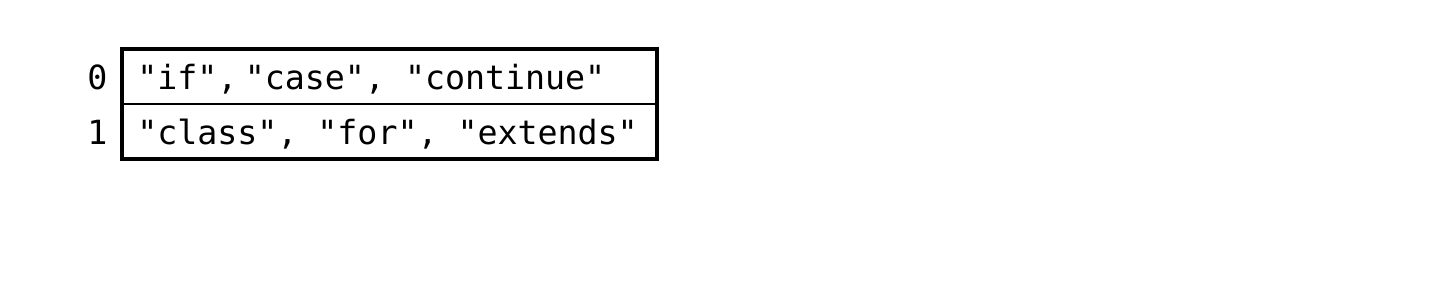
Assume that:
- we’re using keys that are strings
- h(key) = number of characters in key
- we use mod (%) to ensure we get a valid bucket number:
  bucket index = h(key) % number of buckets

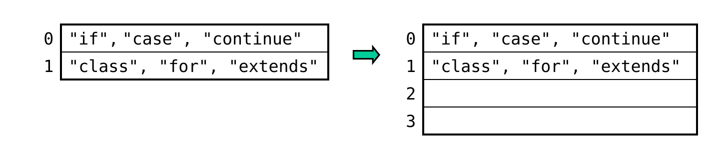
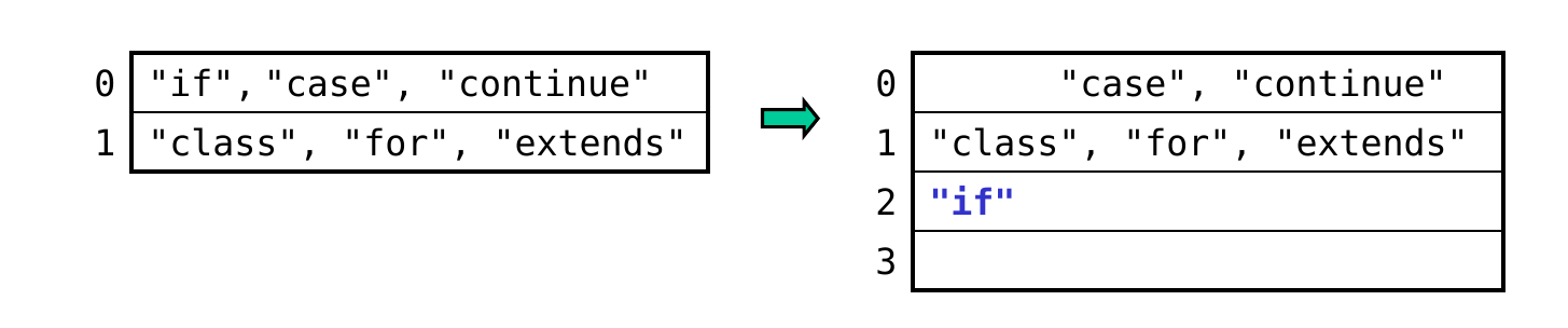
When the hash table gets to be too full:
- double the number of buckets

rehash all existing items. why? % may give a different result