Data Warehousing and OLAP

Part II

Data Science 310

Boston University

Data Warehousing and OLAP Technology

Outline

  • What is a data warehouse? What is OLAP?
  • The Multidimensional Data Model
  • Implementation of Data Cubes
  • Designing a Data Warehouse

Recall: What is a Data Warehouse?

  • A data warehouse is a decision support database that is maintained separately from the organization’s operational database
    • Operational database: personnel / payroll, accounts payable, accounts receivable, orders, inventory, …
    • Data warehouse: none of the above
  • Supports information processing by providing a solid platform of consolidated, historical data for analysis
  • “A data warehouse is a subject-oriented, integrated, time-variant, and nonvolatile collection of data in support of management’s decision-making process.” – W.H. Inmon

Recall: Data Warehouses Support OLAP

  • OLAP: On-Line Analytical Processing
    • Support for decisionmaking
    • Typically involves aggregate operations
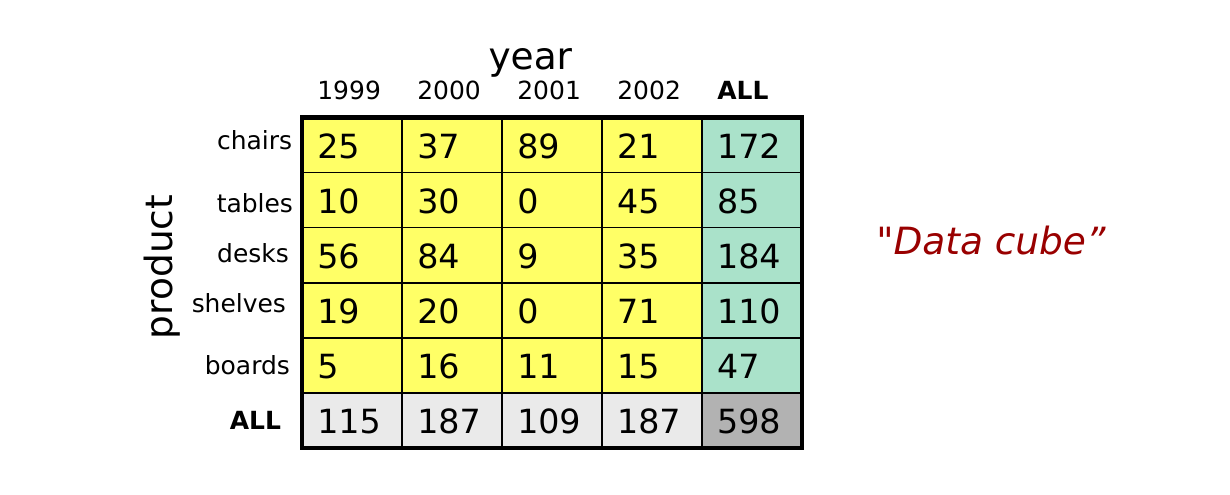
  • Example of an OLAP query (collects counts)
    • Summarize all company sales according to product and year, and further aggregate on each of these dimensions.
Data Warehousing and OLAP Technology

Outline

  • What is a data warehouse? What is OLAP?
  • The Multidimensional Data Model
  • Implementation of Data Cubes
  • Designing a Data Warehouse

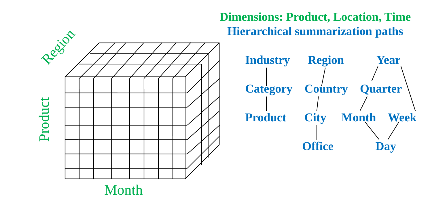
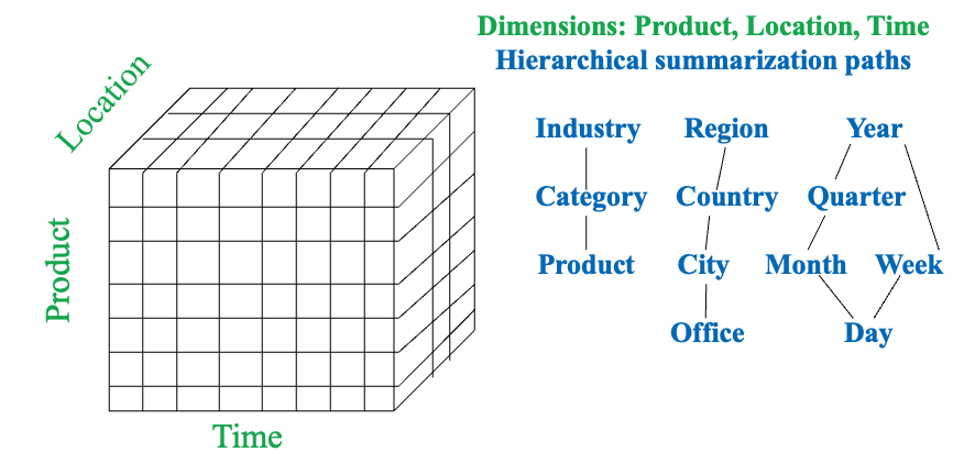
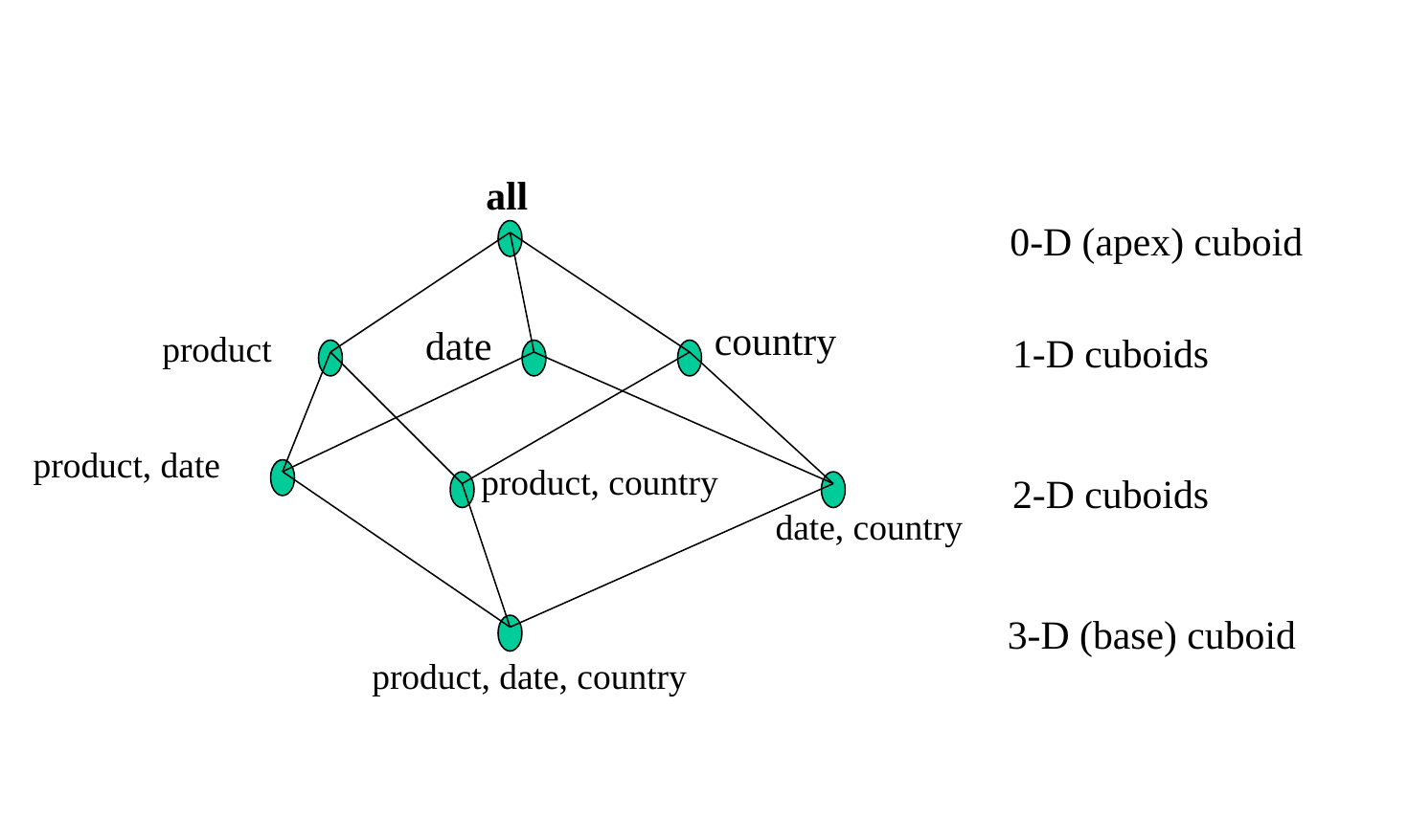
A 3D Data Cube and its Cuboids

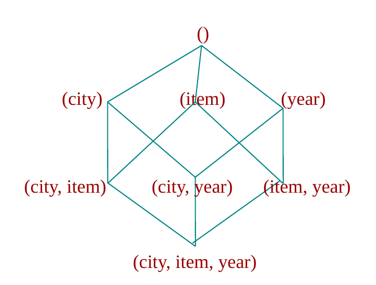
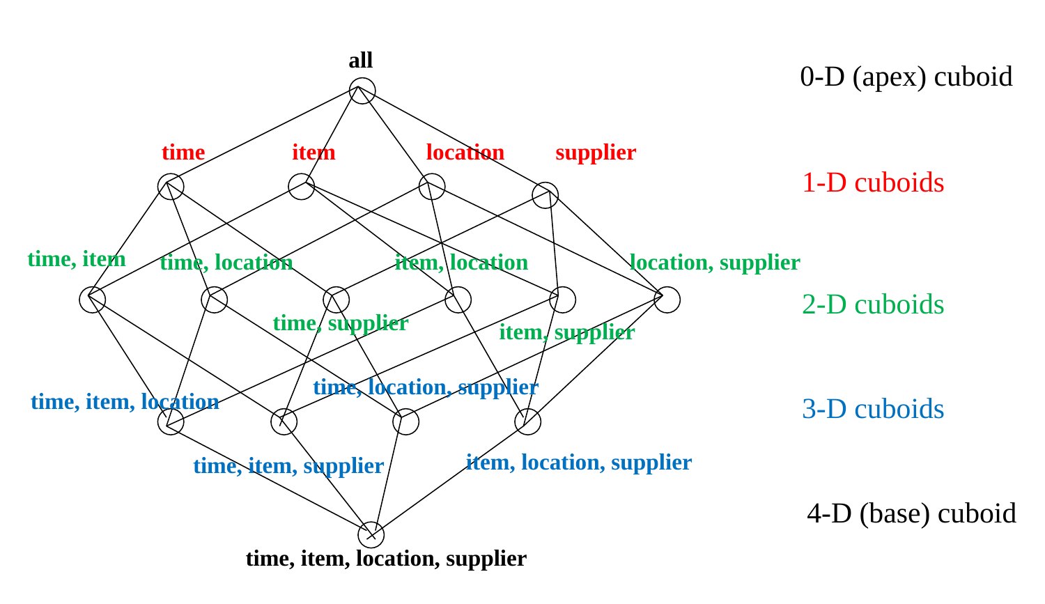
  • The set of cuboids forms a lattice
  • The lattice is a graph showing relationships between cuboids
  • Moving on the lattice corresponds to aggregation or disaggregation
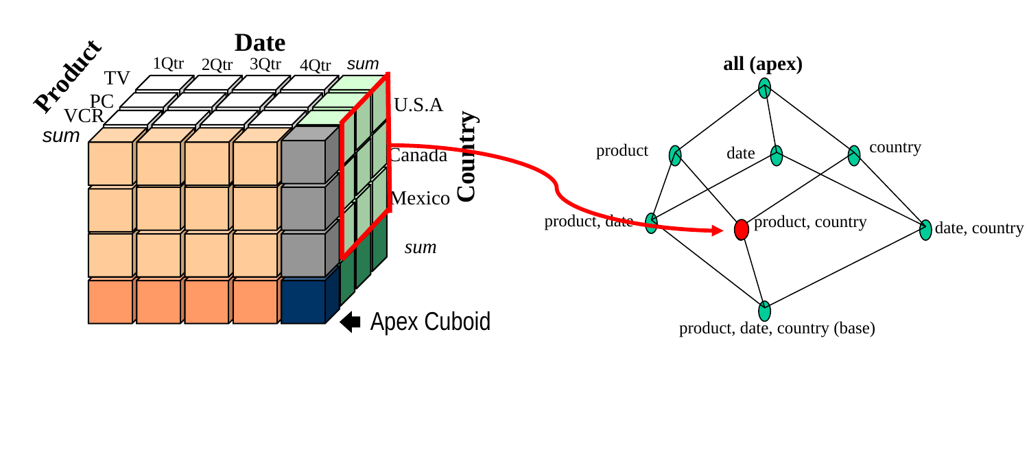
Cuboids Corresponding to the Cube
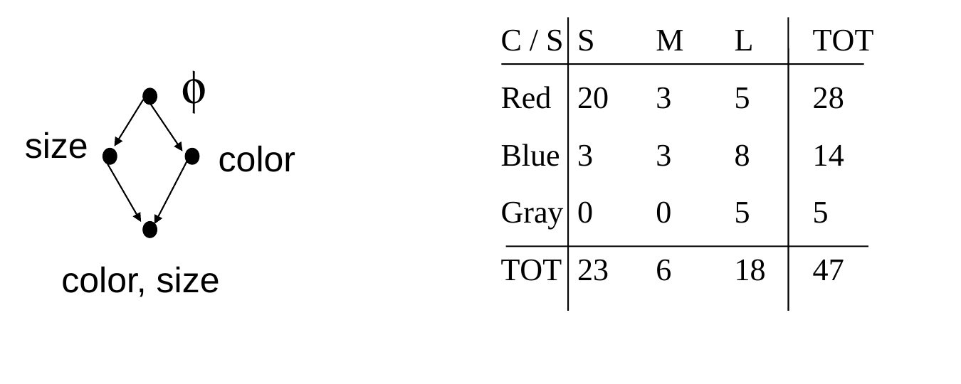
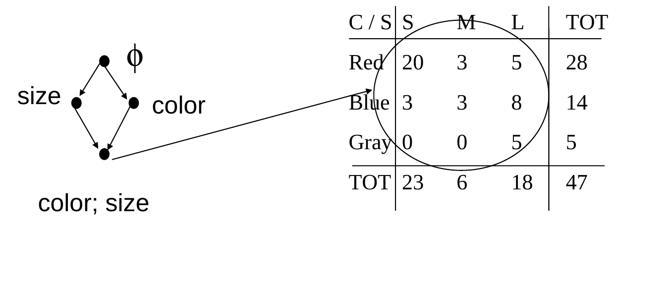
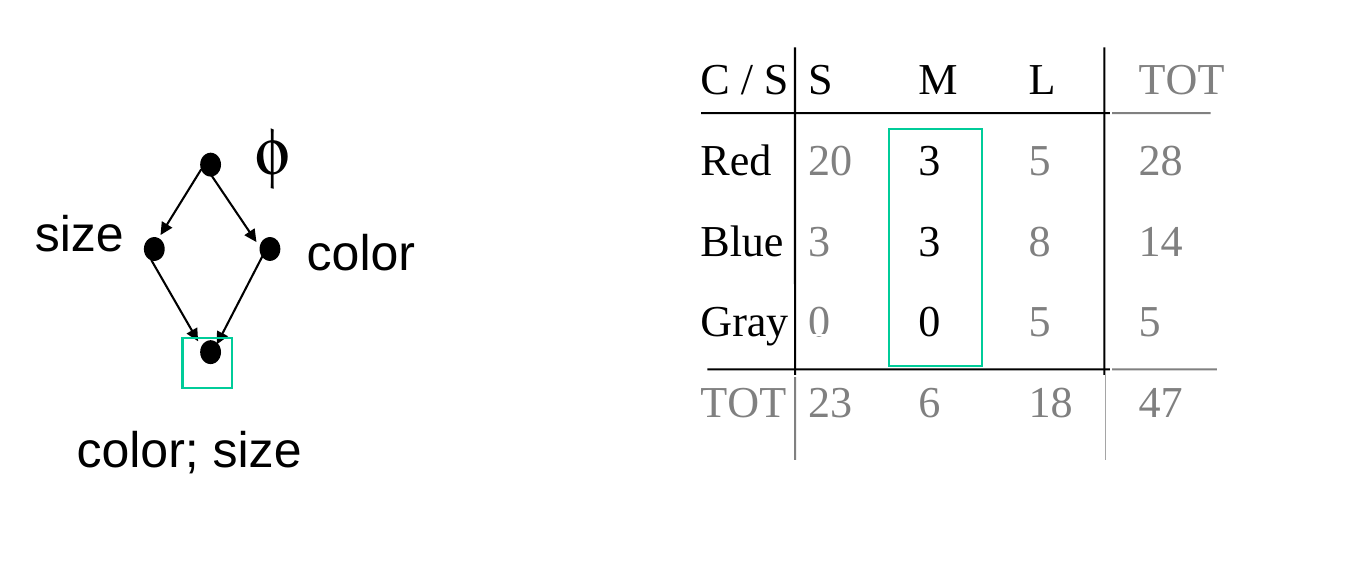
Data Cube Example

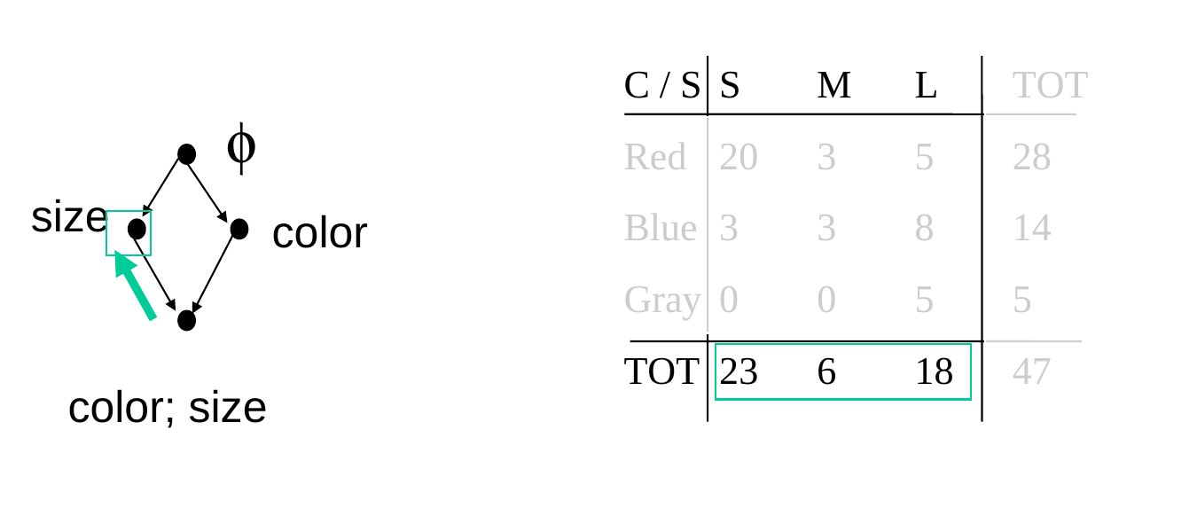
  • ‘color’, ‘size’: DIMENSIONS
  • ‘count’: MEASURE

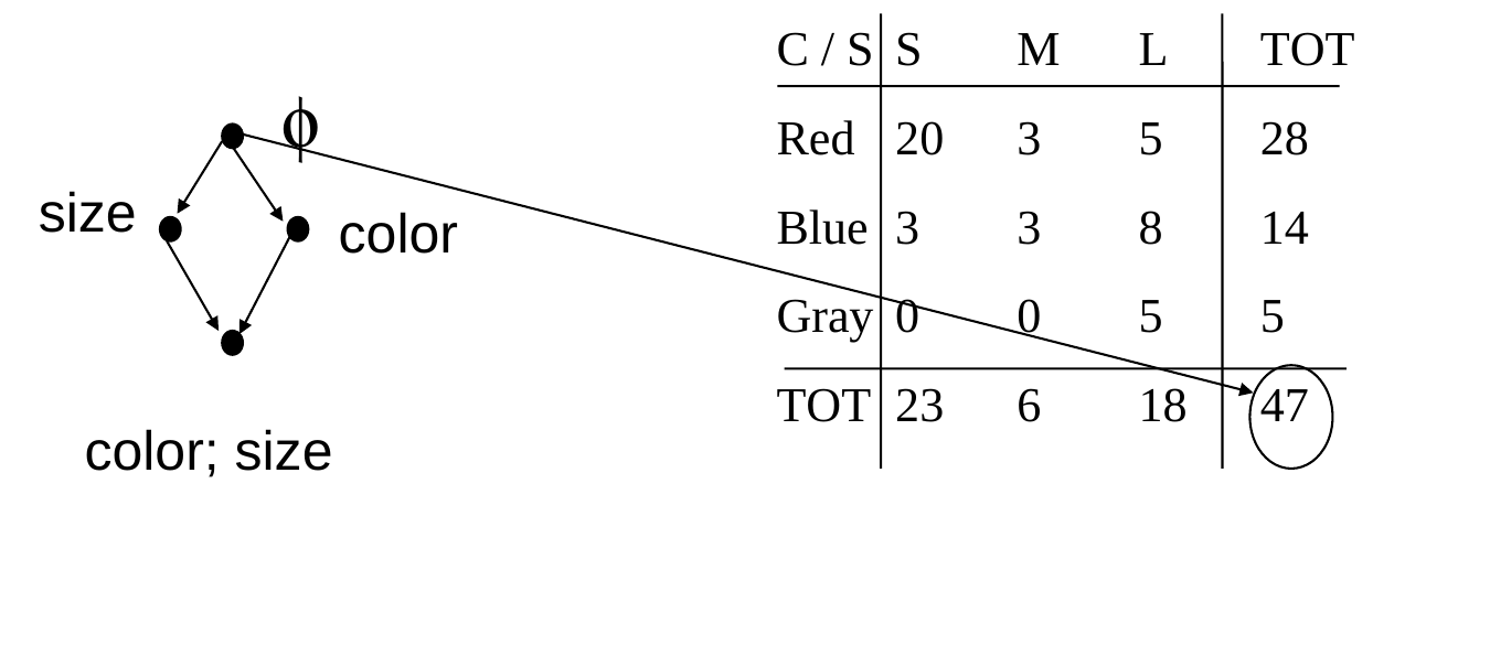
The Apex Cuboid is the Grand Total

  • ‘color’, ‘size’: DIMENSIONS
  • ‘count’: MEASURE

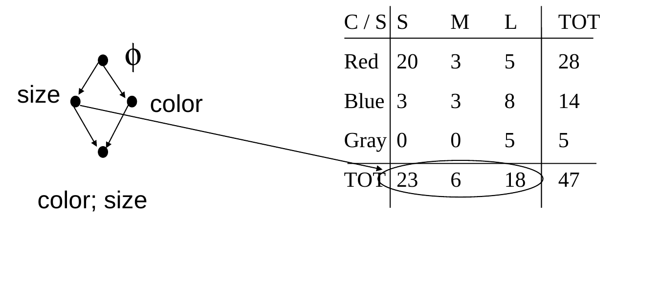
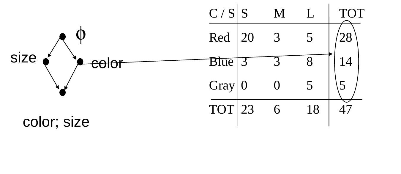
Each 1D Cuboid is a Partial Sum

  • ‘color’, ‘size’: DIMENSIONS
  • ‘count’: MEASURE

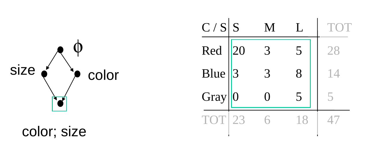
The Detail Data is the Base Cuboid

  • ‘color’, ‘size’: DIMENSIONS
  • ‘count’: MEASURE

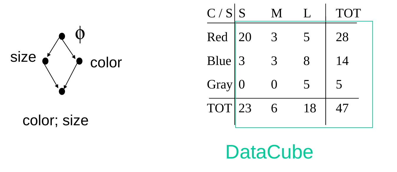
A Data Cube is the Entire Set of Cuboids

  • ‘color’, ‘size’: DIMENSIONS
  • ‘count’: MEASURE

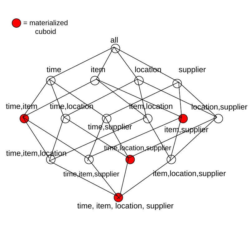
The Lattice of Cuboids of a 4D Cube
Concept Hierarchies

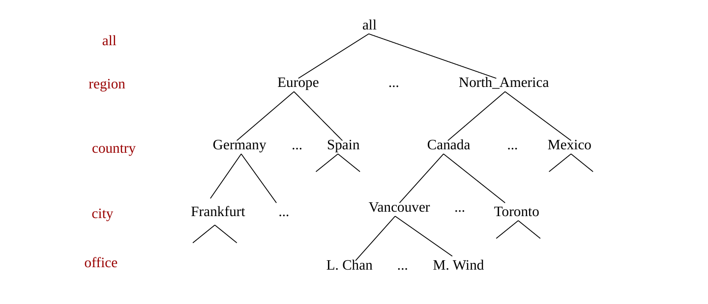
  • A given dimension may have an associated concept hierarchy
  • A concept hierarchy provides another way to aggregate or disaggregate measures
  • This concept hierarchy applies to the location dimension
Summarizing Data

  • A cube may be summarized by removing a dimension
  • Or by climbing in a concept hierarchy

Typical OLAP Operations

  • Browsing between cuboids
    • Roll up (drill-up): summarize data
      • by climbing up the hierarchy or by reducing a dimension
    • Drill down (roll down): reverse of roll-up
      • from higher level summary to lower level summary or detailed data
  • Slice and dice:
    • project and select
  • Pivot (rotate):
    • reorient the cube, visualization, 3D to series of 2D planes.

Example For OLAP Operations

Roll-Up

  • In this example we reduce one dimension
  • It is also possible to climb up in a measure hierarchy
    • Example (product, city) → (product, country)
Drill Down

  • In this example we add one dimension
  • It is possible to move down in a measure hierarchy
    • Example (product, year) → (product, month)
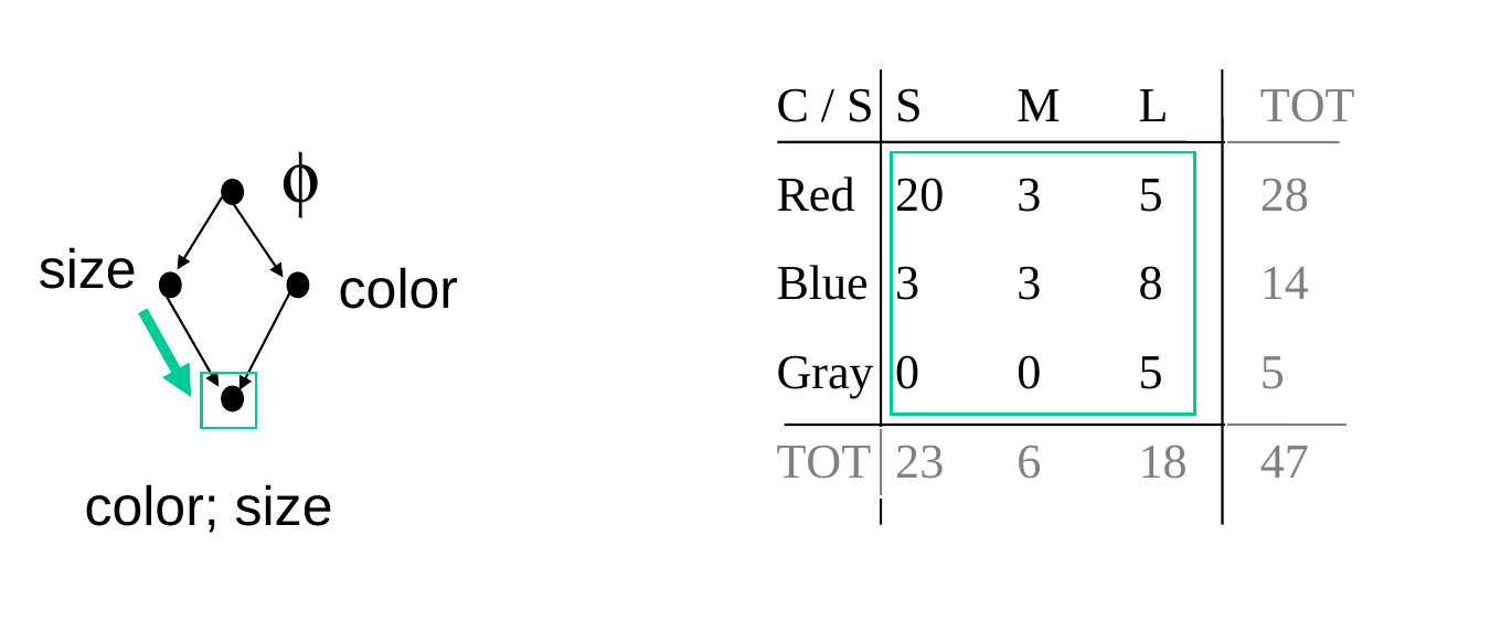
Slice

  • Perform a selection on one dimension

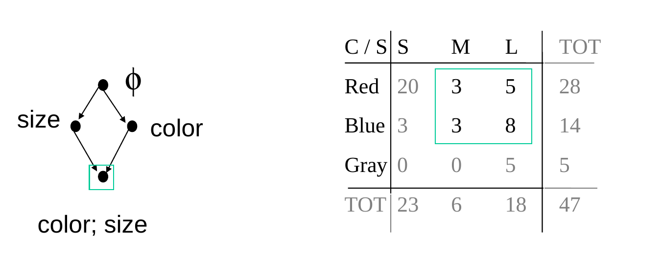
Dice

  • Perform a selection on two or more dimensions
Data Warehousing and OLAP Technology

Outline

  • What is a data warehouse? What is OLAP?
  • The Multidimensional Data Model
  • Implementation of Data Cubes
  • Designing a Data Warehouse

Efficient Data Cube Computation

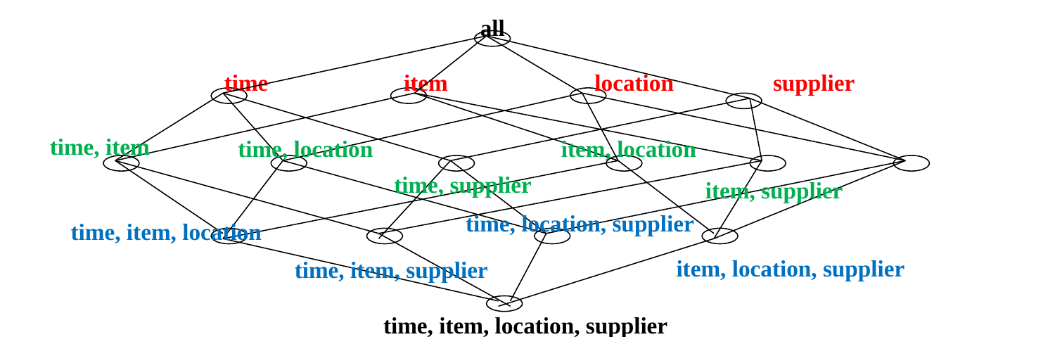
  • As discussed, a data cube may be thought of as a lattice of cuboids
    • Queries will often consist of drill-down or roll-up, ie, moving between cuboids
  • By “materialize” a cuboid we mean to compute it in advance of a query, and maintain it if data changes
    • Materializing a cuboid will speed up queries
  • How many cuboids are in an n-dimensional data cube?
    • If there are no concept hierarchies, there are \(T = 2^{n}\) cuboids
      • Every n-digit binary number represents a cuboid
    • If each dimension has \(L_{i}\) levels, there are \(T = \prod_{i=1}^{n}(L_{i}+1)\) cuboids
  • It may not be feasible or desirable to actually materialize every cuboid

Counting Cuboids

  • In any cuboid, a dimension may be present or absent, and if present, may be aggregated at any level
  • If the dimension is absent, we have summed over all values in that dimension
  • Example:
    • Three dimensions: Product, Location, Time
    • Three levels to Product, four levels to Location, five levels to Time
    • # Cuboids = (4 x 5 x 6) = 120

Materialization Strategies

  • Materialize every cuboid (full materialization)
  • Don’t materialize any cuboids (other than the base)
  • Partial materialization of some cuboids
    • Selection based on size, sharing, access frequency, etc
  • Cuboids are equivalent to the results of GROUP BY operations
Materializing Cuboids

  • Some SQL implementations allow full materialization using CUBE BY
SELECT item, city, year, SUM (amount)
FROM SALES
CUBE BY item, city, year
  • Need compute the following GROUP-Bys:
    • (city, item, year),
    • (city, item), (city, year), (item, year),
    • (city), (item), (year)
    • ( )
  • Example:
SELECT city, item, SUM(amount)
FROM SALES
GROUP BY city, item

Storing Materialized Cuboids

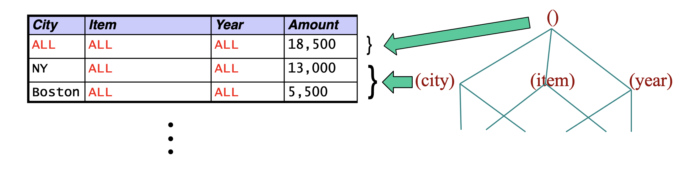
  • Materialized cuboids may be stored in a standard relation by introducing a special value “ALL”
  • Assume our fact table looks like this:
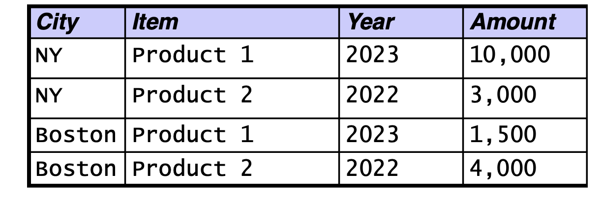
  • Then we can store materialized cuboids as follows:
Retrieving a Cuboid

  • Retrieving a cuboid makes use of the special value ‘ALL’
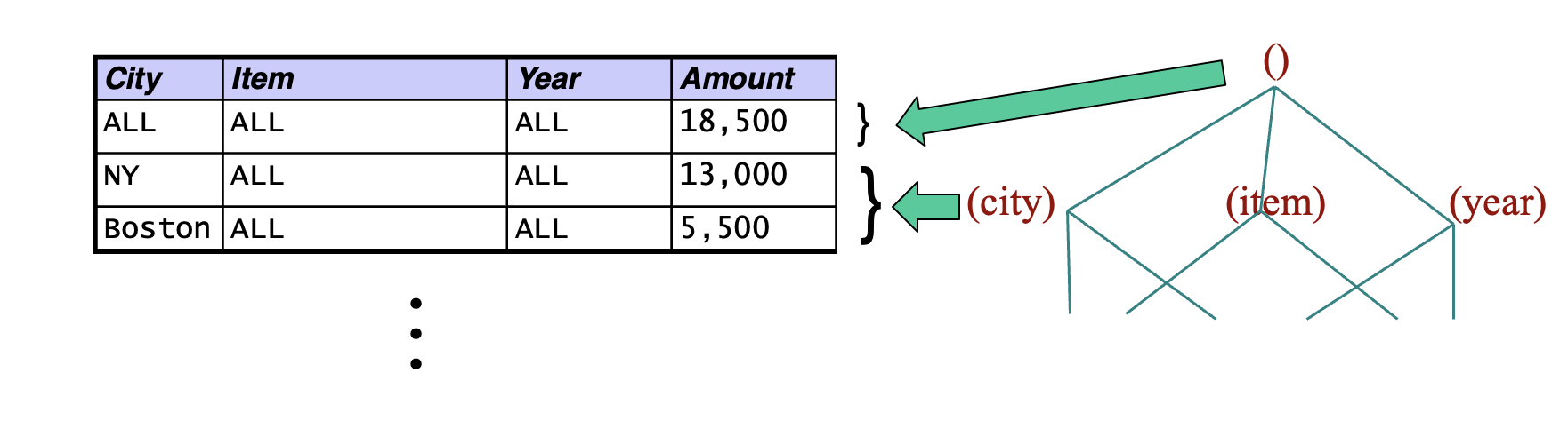
  • To retrieve the (city) cuboid:
SELECT city, item, year, amount
From SALES
WHERE item = 'ALL' and year = 'ALL'

Which Cuboids Should We Materialize?

  • In real-life examples it may not be possible to materialize the whole data cube
  • We have to select the most beneficial cuboids to materialize
  • This depends mainly on the size of the cuboids and their usage by queries
  • Thus to select we need information about
    • the size of cuboids, and
    • the queries and their frequency
  • The base cuboid corresponds to the fact table, which is already materialized.

Retrieving a Non-Materialized Cuboid

  • Retrieving a cuboid that has not been materialized requires a GROUP-BY on a more detailed cuboid
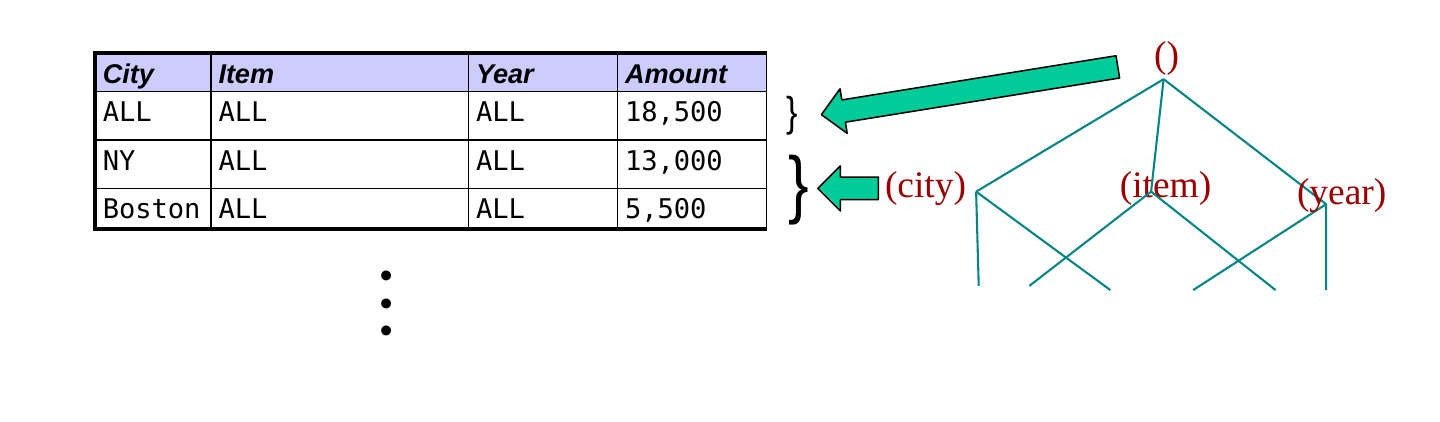
  • To retrieve the (city, item) cuboid:
SELECT  city, item, sum(amount)
From SALES
where city != "ALL" and item != "ALL"
GROUP BY city, item

Why do we need these predicates?

Because other cubes may be materialized!

Example: Which Cuboids Should We Materialize?

  • Example
    • candidate cuboids:
      • (city, item, year) – 100GB (already materialized)
      • (city, item) – 60GB
      • (city, year) – 20GB
      • (item, year) – 1GB
      • (city) – 10GB
      • (item) – 200MB
      • (year) – 30MB
      • (ALL) – 8 bytes
    • queries (with equal probability)
      • Q1: total sales per (item, year)
      • Q2: total sales per (item)
      • Q3: total sales per (year)

Which views should we materialize if the available space is:

  1. 10GB
  2. 1GB
  3. 100MB

Case 1

  • Case 1: Available space = 10GB
    • We can materialize all three views (item, year), (item), and (year)
    • The cost of Q1 is reading 1GB
    • The cost of Q2 is reading 200MB
    • The cost of Q3 is reading 30MB
    • Average query cost = (1230 MB) / 3 = 410 MB /query

Case 2

  • Case 2: Available space = 1GB
  • We have two choices:
    • materialize (item, year) using 1GB
      • Q1 costs 1GB, Q2 costs 1GB, Q3 costs 1GB
      • Average query cost = 1GB
    • materialize (item) and (year) using 230 MB
      • Q1 costs 100 GB, Q2 costs 200 MB, Q3 costs 30 MB
        • Why does Q1 cost 100 GB?
      • Average query cost = (100.230 GB) / 3 = 34 GB
  • First choice is better than the second!

Case 3

  • Case 3: Available space = 100MB
  • We can only materialize (year)
    • Q1 costs 100 GB
    • Q2 costs 100 GB
    • Q3 costs 30 MB
    • Average query cost = (200.030 MB) / 3 = 67 GB

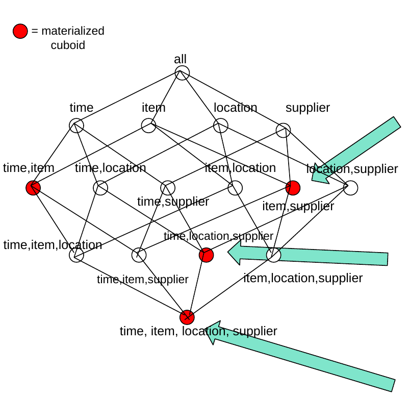
Practice: Retrieving Cuboids

Given the cuboids that are materialized, how would you retrieve the following cuboids?

  • Q1: (time, item)
  • Q2: (supplier)
  • Q3: (location)

Q1: (time, item)

This cuboid is materialized.

So we can simply query it:

SELECT time, item, location, supplier, amount
FROM table
WHERE location = 'ALL' and supplier = 'ALL'

Q2: supplier

We have a number of options:

SELECT supplier, sum(amount)
WHERE location = 'ALL' and time = 'ALL'
GROUP BY supplier

or:

SELECT supplier, sum(amount)
WHERE item = 'ALL'
GROUP BY supplier

or:

SELECT supplier, sum(amount)
GROUP BY supplier

Which is most efficient?

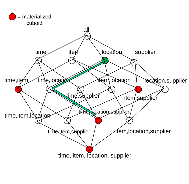
Q3: (location)

Strategy to find most efficient query:

  • Find the closest materialized predecessor in the cuboid lattice
  • Base your query on that cuboid
SELECT location, sum(amount)
FROM table
WHERE item = 'ALL'
GROUP BY location

More Practice: Retrieving Cuboids

Given the cuboids that are materialized, how would you retrieve the following cuboids?

  • Q4: (time, supplier)
  • Q5: (item)

Data Warehousing and OLAP Technology

Outline

  • What is a data warehouse? What is OLAP?
  • The Multidimensional Data Model
  • Implementation of Data Cubes
  • Designing a Data Warehouse

Reminder: Goal of a Data Warehouse

  • “A data warehouse is a subject-oriented, integrated, time-variant, and nonvolatile collection of data in support of management’s decision-making process.”
  • A data warehouse is a decision support database that is maintained separately from the organization’s operational database

The DW Design Process

  • Use requirements specifications and consult with analysts to select
    • The central theme of the analysis
      • For example, sales
    • The measures on the central theme
      • For example, sum(dollars)
    • The dimensions used by analytical processing
    • The attributes and hierarchies of the dimensions
  • Design the schema
  • Clean, transform, and integrate information
    • Drawing from operational databases

Example: Large Company Selling Engine Parts

  • Operational Database 1 (Los Angeles)
    • employee(id, name, dept, lot, salary, age)
    • department(id name, type, manager_id)
    • part(id, name, type, brand, manufacturer, color)
    • customer(id, name, type, age, city, state, zip, tel)
    • sales(id, part_id, customer_id, quantity, price)
  • Operational Database 2 (New York)
    • employee(id, ename, dept_id, salary, age)
    • department(id, name, type, manager)
    • part(id, title, type, brand, manufacturer, color)
    • customer(id, name, type, zip, tel)
    • location(zip, city_id)
    • city(city_id, state, country)
    • sales(id, part_id, customer_id, quantity, price)
  • Notice variation in attribute names, table structure, normalization!
  • Notice that some tables are of interest for analyzing company’s business, some not

Determining the Basic Features

  • After consultation with analysts, we observe that a theme for the DW should be sales
  • Specifically, we want to analyze total sales in dollars, and average prices of sold units with respect to time, part, and customer.
  • We select the basic features of the DW:
    • Central theme(s): sales
    • Measures: sum(sales_in_dollars), avg(price_sold_units)
    • Dimensions: time, part, customer

Selecting Hierarchies

  • Next we determine dimension hierarchies
  • This too is done in consultation with analysts
  • We determine that hierarchies should be:
    • Time: day, week, month, quarter, year
    • Part: name, type, color, brand, manufacturer
    • Customer: name, type, city, state, country
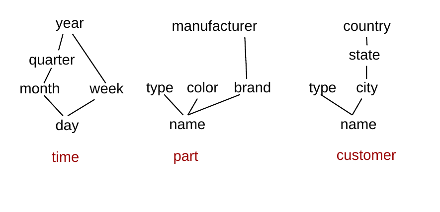
Q: how many cuboids will there be in this data cube?

A: 6 x 6 x 6 = 216

Data Sufficiency

  • Does all the needed information exist in the operational databases?
  • In this example, we determine that all requested attributes exist, except for time
  • We determine that we will obtain time information by accessing the transaction logs of the operational databases.

Design the DW schema

  • In this example, we decide to use a star schema
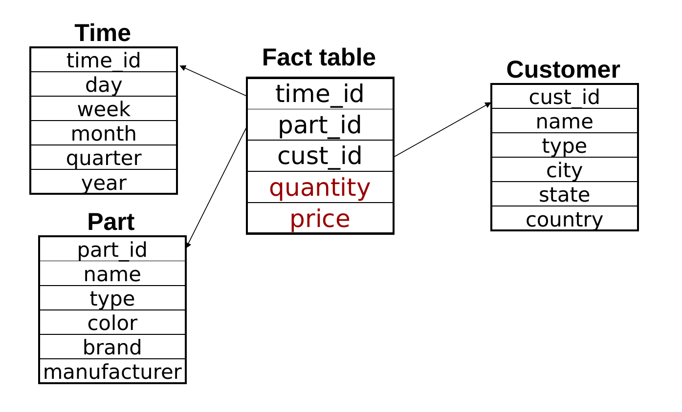
  • We determine that we only need quantity and (unit) price to derive
    • sum(sales_in_dollars) = quantity*price
    • avg(price_sold_units) = Σ(quantity*price)/ Σ(quantity)

Data Integration

  • Operational Database 1 (Los Angeles)
    • employee(id, name, dept, lot, salary, age)
    • department(id name, type, manager_id)
    • part(id, name, type, brand, manufacturer, color)
    • customer(id, name, type, age, city, state, zip, tel)
    • sales(id, part_id, customer_id, quantity, price)
  • Operational Database 2 (New York)
    • employee(id, ename, dept_id, salary, age)
    • department(id, name, type, manager)
    • part(id, title, type, brand, manufacturer, color)
    • customer(id, name, type, zip, tel)
    • location(zip, city_id)
    • city(city_id, state, country)
    • sales(id, part_id, customer_id, quantity, price)
  • Convert attribute names and types
    • eg, since part.name = part.title
  • Join tables if necessary
    • Join customer, location, city from New York DB
  • Derive time if not present
    • Transaction logs from sales table
  • Complete missing values
    • Los Angeles DB does not record customer country because all customers are from US. In the data taken from LA DB, set country value to “US”
  • Ignore irrelevant tables and attributes
    • Tables employee, department are ignored
    • Attributes zip, tel, id are ignored

Materialization

  • Finally, decide which cuboids to materialize
  • Base this on space available and expected mix of queries